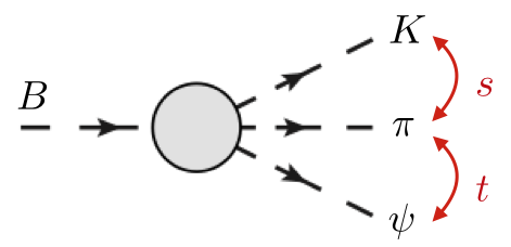
 This page concerns the kinematics of the reaction $B \to K \pi \psi$
from the publication [Mik18a] .
A brief description of the formalism is given in the Formalisms section.
Please see the publication [Mik18a] for further details.
Both side of the sum rules are compared interactively in the Simulation section.
The codes can be downloaded in Resources section.
Formalism
| $A_k^{(\sigma)}$ | | | $I^G$ | $P(-1)^J$ | $\tau$ | $J^{PC}$ | | | lightest meson | ||||||||||
| $--$ | | | $--$ | $----$ | $--$ | $-----$ | | | $------$ | $A_{3}^{(+)}$ | | | $0^-$ | $-1$ | $+1$ | $(1,3,\ldots)^{+-}$ | | | $\omega_2(-)$ | ||
| $A_{3}^{(-)}$ | | | $1^-$ | $-1$ | $-1$ | $(2,4,\ldots)^{-+}$ | | | $a_1(1260)$ | ||||||||||
| $--$ | | | $--$ | $----$ | $--$ | $-----$ | | | $------$ |
| $(\sigma)$ | | | $(0)$ | $(+)$ | $(-)$ | | | values |
| $--$ | | | $----$ | $----$ | $----$ | | | $------$ |
| $B_1^{(\sigma)}$ | | | $-\frac{1}{2}\frac{eg}{2 M}$ | $-\frac{1}{2}\frac{eg}{2 M}$ | $-\frac{1}{2}\frac{eg}{2 M}$ | | | $e = 0.303$ |
| $B_2^{(\sigma)}$ | | | $\frac{1}{t-\mu^2}\frac{eg}{2 M}$ | $\frac{1}{t-\mu^2}\frac{eg}{2 M}$ | $\frac{1}{t-\mu^2}\frac{eg}{2 M}$ | | | $g = 13.54$ |
| $B_3^{(\sigma)}$ | | | $\frac{\kappa_p+\kappa_n}{4 M}\frac{eg}{2 M}$ | $\frac{\kappa_p-\kappa_n}{4 M}\frac{eg}{2 M}$ | $\frac{\kappa_p-\kappa_n}{4 M}\frac{eg}{2 M}$ | | | $\kappa_p = 1.78$ |
| $B_4^{(\sigma)}$ | | | $\frac{\kappa_p+\kappa_n}{4 M}\frac{eg}{2 M}$ | $\frac{\kappa_p-\kappa_n}{4 M}\frac{eg}{2 M}$ | $\frac{\kappa_p-\kappa_n}{4 M}\frac{eg}{2 M}$ | | | $\kappa_n = -1.91$ |
| $--$ | | | $----$ | $----$ | $----$ | | | $------$ |
Model
Every isobar is simple Breit-Wigner \begin{equation} BW(x, m, g) = \frac{c}{m^2 - x - i mg} \end{equation}
References
[Mik18a]
M. Mikhasenko, A. Pilloni,, J. Nys, M. Albaladejo, C. Fernandez-Ramirez,
A. Jackura, V. Mathieu, N. Sherill, T. Skwarnicki and A. P. Szczepaniak
``What is the right formalism to search for resonances?,''
arXiv:1712.02815 [hep-ph],
Eur. Phys. J. C78 (2018) 229
Resources
- Publications: [Mik18a]
- C/C++: FESR-PiPhot-Low.c,
- Input file: input.txt, couplings.txt
- Contact person: Vincent Mathieu (mathieuv.at.indiana.edu)
- Last update: June 2018
- FESR-PiPhot-Low.c:
- Read_Multipoles reads the multipoles from files.
- FESR-PiPhot-Regge.c:
- FESR_Regge returns the FESR at fixed $t$.
- Ai_Regge returns the scalar amplitudes at fixed $t$ and $s$.
- DSig_Regge returns the differential cross section at fixed $t$ and $s$.
- Pol_Regge returns the polarization observables at fixed $t$ and $s$.
- Simulation-param.txt
Elab tmin tmax dt cutoff k1 k2 wmin wmax dw t0
- Elab: Lab energy for printing the observables for high energy
- tmin tmax dt: interval in t for the FESR
- wmin wmax dw: interval in $W=\sqrt{s}$ for printing Ai
- t0: print Ai at t = t0
- cutoff: W-max for the FESR
- k1 k2: moments of the FESR
- Trajectories.txt
Intercept and slopes of 10 trajectories. Only the 8 first are used in this model. - Residues.txt
Parameters of the 12x2 residues $\beta(t)$.
Each amplitudes contains 2 contribution, the leading Regge pole and a sub-leading contribution.
In this model, the unnatural amplitude has only one contribution. The parameters of their sub-leading pole are set to zero.
Each line is $j$, $\kappa$, $\delta$, $\beta_0$, $b$, $\gamma_1$, $\gamma_2$.
Simulation
The code compute both side of the FESR Eq. \eqref{eq:FESR} with the moment $k_1$ (odd amplitudes) and $k_2$ (even amplitudes).The user can choose the moments $k_{1,2}$. They must be even positive integers.
$k_1$ must be odd and $k_2$ must be even.
The suggested cutoff is $E^\text{lab}_\text{max}$ is 2 GeV. The SAID model can be used up to 2.4 GeV and MAID up to 2.0 GeV
Note that imposing a cutoff above the range of validity of a solution might lead to misleading results.
The limit of validity of the models can be read from the partial waves files.
One can print the observables (differential cross section and $\Sigma,T,R$ asymmetries) using the Regge model.
The default value to compute the observables is $E^\text{lab}_\gamma = 9$ GeV.
The default $t$ range for the observables and the FESR is $t\in [-1,0]$ GeV$^2$.
The kinematical quentities are expressed in GeV.
The parameters (trajectories and residues) of the model can be changed. The defaults values are taken from [Mat18b] .