A Complete Example

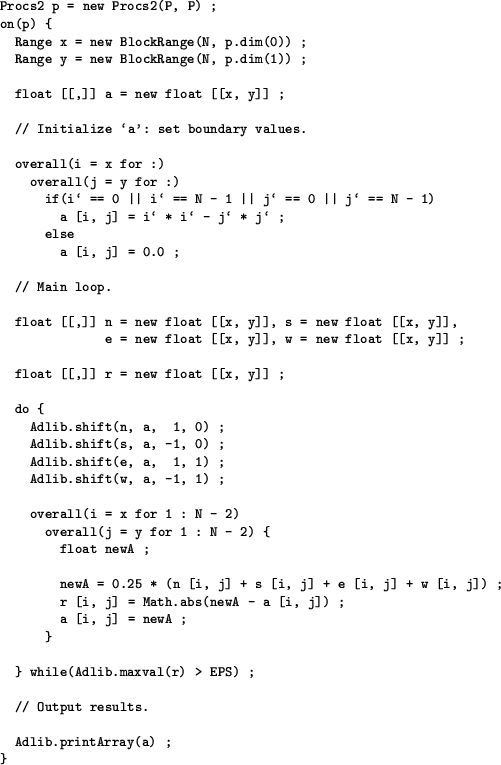
The example of Figure 2.7 only uses language features introduced in the preceding sections. It introduces two new library functions.

Figure 2.7: Solution of Laplace equation by Jacobi relaxation.

The problem is a very well-known one: solution of the two-dimensional Laplace equation with Dirichlet boundary conditions by the iterative Jacobi relaxation method ^2.7. The boundary conditions of the equation are fixed by setting edge elements of an array. These elements don't change throughout the computation. The solution for the interior region is obtained by iteration from some arbitrary starting values (zero, here). A single iteration involves replacing each interior element by the average of its neighbouring values. A similar update was already discussed in section 2.3. Here we put it in the context of a working program.

The initialization is done with a pair of nested overall constructs. Inside, a conditional tests if we are on an edge of the array. If so, the element values are set to some chosen expression--the boundary function. Otherwise we zero an interior element. As discussed at the end of the last section we, apply the operator ` to bound locations to get the global loop index.

Notice that one can freely use ordinary Java constructs like if inside an overall construct. HPJava distributed control construct are true, compositional control constructs. They differ in this respect from the HPF forall construct, which has restrictive rules about what kind of statement can appear in its body.

If preferred, the edges could have been initialized using at constructs:

    at(i = x [0])
      overall(j = y for :)
        a [i, j] = i` * i` - j` * j` ;
    
    at(i = x [N - 1])
      overall(j = y for :)
        a [i, j] = i` * i` - j` * j` ;
    
    at(j = y [0])
      overall(i = x for :)
        a [i, j] = i` * i` - j` * j` ;
    
    at(j = y [N - 1])
      overall(i = x for :)
        a [i, j] = i` * i` - j` * j` ;

with the interior initialized separately using nested overall constructs:

    overall(i = x for 1 : N - 2)
      overall(j = y for 1 : N - 2)
        a [i, j] = 0.0

This version is more long-winded but potentially more efficient, because it simplifies the inner loop bodies, improving the scope for compiler optimization.

The body of the main loop contains shift operations and nested overall loops. The body of the inner loop is slightly more complicated than the version in figure 2.5 because it saves changes to the main array in a separate array r.

Note the declaration of the float temporary newA inside the body of the parallel loop. This is perfectly good practise. The temporary is just an ordinary scalar Java variable--the HPJava translator doesn't treat it specially. Also note the call to a Java library function abs inside the loop. As we have emphasized, any normal Java operation is allowed inside an HPJava distributed control construct.

The main loop terminates when the largest change in any element is smaller than some predefined value EPS. The collective library function maxval finds the largest element of distributed array, and broadcasts its value to all processes that call the function. [Need to initialize edges of r to zero.]

Finally a collective library function printArray prints a formatted versions of the array on the standard output stream.